GitHub Newsletter Discord

Version: 0.6.1.3

R-NSGA-III

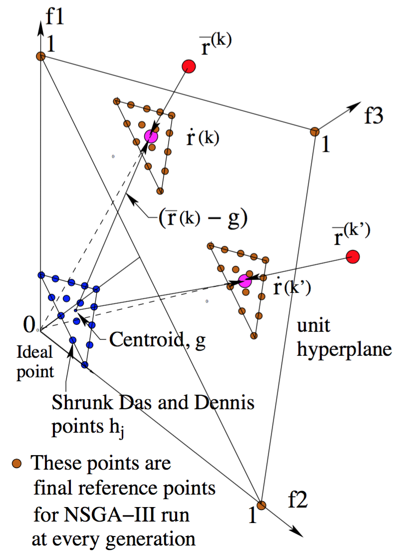
Implementation details of this algorithm can be found in [10]. The reference lines that should be used by this algorithm must be defined before it is executed. Commonly, the Das-Dennis method (implemented in UniformReferenceDirectionFactory) is used to sample reference directions uniformly.

To generate the reference directions refer to the R-NSGA-III paper where the following procedure is laid out in detail.

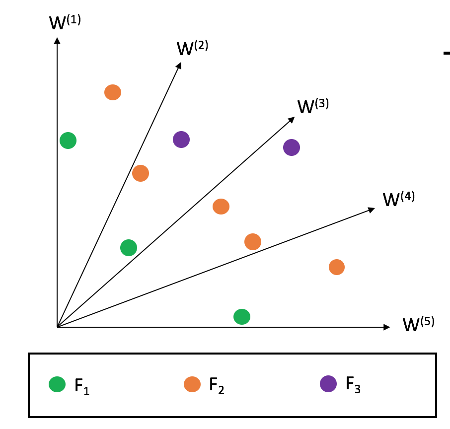
The algorithm follows the general NSGA-III procedure with a modified survival selection operator. First, the non-dominated sorting is done as in NSGA-III.

Second, from the splitting front (final front), some solutions need to be selected. Solutions are associated with reference directions based on perpendicular distance, then solutions with smaller ASF values are preferred by selecting solutions from the underrepresented reference direction first. For this reason, when this algorithm converges, each reference line seeks to find a good representative non-dominated solution.

Example

import numpy as np

from pymoo.algorithms.moo.rnsga3 import RNSGA3
from pymoo.problems import get_problem
from pymoo.optimize import minimize
from pymoo.visualization.scatter import Scatter

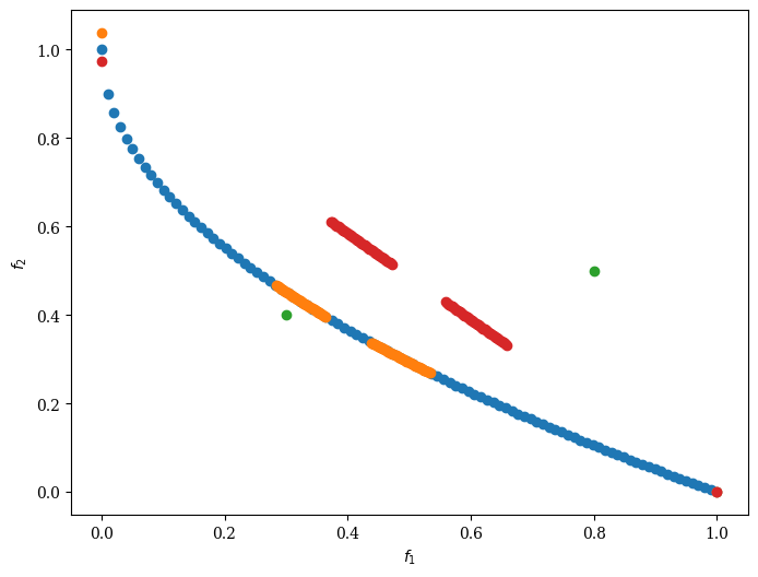
problem = get_problem("zdt1")
pf = problem.pareto_front()

# Define reference points
ref_points = np.array([[0.3, 0.4], [0.8, 0.5]])

# Get Algorithm
algorithm = RNSGA3(
    ref_points=ref_points,
    pop_per_ref_point=50,
    mu=0.1)

res = minimize(problem,
               algorithm=algorithm,
               termination=('n_gen', 300),
               pf=pf,
               seed=1,
               verbose=False)

reference_directions = res.algorithm.survival.ref_dirs

plot = Scatter()
plot.add(pf, label="pf")
plot.add(res.F, label="F")
plot.add(ref_points, label="ref_points")
plot.add(reference_directions, label="ref_dirs")
plot.show()

<pymoo.visualization.scatter.Scatter at 0x11fd12780>

from pymoo.util.reference_direction import UniformReferenceDirectionFactory

# Get problem
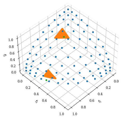
problem = get_problem("dtlz4", n_var=12, n_obj=3)

# Define reference points and reference directions
ref_points = np.array([[1.0, 0.5, 0.2], [0.3, 0.2, 0.6]])
ref_dirs = UniformReferenceDirectionFactory(3, n_points=91).do()
pf = problem.pareto_front(ref_dirs)

# Get Algorithm
algorithm = RNSGA3(
    ref_points=ref_points,
    pop_per_ref_point=91,
    mu=0.1)

res = minimize(problem,
               algorithm,
               termination=('n_gen', 300),
               pf=pf,
               seed=1,
               verbose=False)


plot = Scatter()
plot.add(pf, label="pf")
plot.add(res.F, label="F")
plot.add(ref_points, label="ref_points")
plot.show()

<pymoo.visualization.scatter.Scatter at 0x11fd81790>

API

class pymoo.algorithms.moo.rnsga3.RNSGA3(self, ref_points, pop_per_ref_point, mu=0.05, sampling=FloatRandomSampling(), selection=TournamentSelection(func_comp=comp_by_cv_then_random), eliminate_duplicates=True, n_offsprings=None, **kwargs)

Parameters

ref_pointsnumpy.array

Reference Points (or also called Aspiration Points) as a numpy.array where each row represents a point and each column a variable (must be equal to the objective dimension of the problem)

pop_per_ref_pointint

Size of the population used for each reference point.

mufloat

Defines the init_simplex_scale of the reference lines used during survival selection. Increasing mu will result having solutions with a larger spread.

n_offspringsint (default: None)

Number of offspring that are created through mating. By default n_offsprings=None which sets the number of offsprings equal to the population size. By setting n_offsprings=1 a, so called, steady-state version of an algorithm can be achieved.

samplingSampling, Population, numpy.array

The sampling process defines the initial set of solutions which are the starting point of the optimization algorithm. Here, you have three different options by passing

(i) A Sampling implementation which is an implementation of a random sampling method.

(ii) A Population object containing the variables to be evaluated initially OR already evaluated solutions (F needs to be set in this case).

(iii) Pass a two dimensional numpy.array with (n_individuals, n_var) which contains the variable space values for each individual.

selectionSelection

This object defines the mating selection to be used. In an evolutionary algorithm each generation parents need to be selected to produce new offsprings using different recombination and mutation operators. Different strategies for selecting parents are possible e.g. selecting them just randomly, only in the neighborhood, using a tournament selection to introduce some selection pressure, …

crossoverCrossover

The crossover has the purpose of create offsprings during the evolution. After the mating selection the parents are passed to the crossover operator which will dependent on the implementation create a different number of offsprings.

mutationMutation

Some genetic algorithms rely only on the mutation operation. However, it has shown that increases the performance to perform a mutation after creating the offsprings through crossover as well. Usually the mutation operator needs to be initialized with a probability to be executed. Having a high probability of mutation will most of the time increase the diversity in the population.

eliminate_duplicatesbool

The genetic algorithm implementation has a built in feature that eliminates duplicates after merging the parent and the offspring population. If there are duplicates with respect to the current population or in the offsprings itself they are removed and the mating process is repeated to fill up the offsprings until the desired number of unique offsprings is met.

<< U-NSGA-III

MOEA/D >>