Part I: A Constrained Bi-objective Optimization Problem#
In the following, we investigate exemplarily a bi-objective optimization with two constraints. We have tried to select a suitable optimization problem with enough complexity for demonstration purposes, but not too difficult to lose track of the overall idea. Its definition is given by:
As already discussed in the Preface, let an optimization problem be defined by:
\begin{align} \begin{split} \min \quad& f_{m}(x) \quad \quad \quad \quad m = 1,..,M \\[4pt] \text{s.t.} \quad& g_{j}(x) \leq 0 \quad \; \; \, \quad j = 1,..,J \\[2pt] \quad& h_{k}(x) = 0 \quad \; \; \quad k = 1,..,K \\[4pt] \quad& x_{i}^{L} \leq x_{i} \leq x_{i}^{U} \quad i = 1,..,N \\[2pt] \quad& x \in \Omega \end{split} \end{align}
The example problem to be solved in this getting started guide is given by:
\begin{align} \begin{split} \min \;\; & f_1(x) = 100 \,(x_1^2 + x_2^2) \\ \max \;\; & f_2(x) = -(x_1-1)^2 - x_2^2 \\[1mm] \text{s.t.} \;\; & g_1(x) = 2 \, (x_1 - 0.1) \, (x_1 - 0.9) \leq 0\\ & g_2(x) = 20 \, (x_1 - 0.4) \, (x_1 - 0.6) \geq 0\\[1mm] & -2 \leq x_1 \leq 2 \\ & -2 \leq x_2 \leq 2\\[1mm] & x \in \mathbb{R} \end{split} \end{align}
The problem consists of two objectives (\(M=2\)) where \(f_1(x)\) is minimized and \(f_2(x)\) maximized. The optimization is subject to two inequality constraints (\(J=2\)) where \(g_1(x)\) is formulated as a less than and \(g_2(x)\) as a greater than constraint. The problem is defined with respect to two variables (\(N=2\)), \(x_1\) and \(x_2\), both in the range \([-2,2]\). The problem does not contain any equality constraints (\(K=0\)).
Note
Next, we derive the optimum for the given optimization problem. It is worth pointing out that this is not a requirement for pymoo and is just done for verification purposes here. Moreover, this is a valuable exercise to understand the design and objective space mapping.
Let us analyze where the Pareto-optimal solutions have to lie. The first objective \(f_1\) is minimized at \((0,0)\), whereas the second object \(f_2\) at \((1, 0)\). Because both functions are of quadratic nature, the optimum is given by a straight line between the two optima. This means all Pareto-optimal solutions (ignoring the constraints for now) have in common that \(x_2=0\) and \(x_1 \in (0,1)\). The first constraint only relies on \(x_1\) and is satisfied if \(x_1 \in (0.1,0.9)\). The second constraint \(g_2\) is satisfied for \(x_1 \in (-\infty,0.4) \lor x_1 \in (0.6,\infty)\). This means analytically, the pareto-optimal set is given by \(PS = \{(x_1, x_2) \,|\, (0.1 \leq x_1 \leq 0.4) \lor (0.6 \leq x_1 \leq 0.9) \, \land \, x_2 = 0\}\).
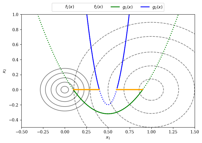
The figure below shows the problem’s functions in the design space and might help to see the relationship between the functions intuitively. The contour lines of the objective function \(f_1(x)\) is represented by a solid and \(f_2(x)\) by a dashed line. The constraints \(g_1(x)\) and \(g_2(x)\) are parabolas which intersect the \(x_1\)-axis at \((0.1, 0.9)\) and \((0.4, 0.6)\). A thick orange line illustrates the Pareto-optimal set. When considering both constraints together, the Pareto-set shown in orange is split into two parts as analytically derived above.
[1]:
import numpy as np

X1, X2 = np.meshgrid(np.linspace(-2, 2, 500), np.linspace(-2, 2, 500))

F1 = 100 * (X1**2 + X2**2)
F2 = (X1-1)**2 + X2**2

G1 = 2 * (X1[0] - 0.1) * (X1[0] - 0.9)
G2 = 20 * (X1[0] - 0.4) * (X1[0] - 0.6)

import matplotlib.pyplot as plt
plt.rc('font', family='serif')

levels = np.array([0.02, 0.1, 0.25, 0.5, 0.8])
plt.figure(figsize=(7, 5))
CS1 = plt.contour(X1, X2, F1, 10 * levels, colors='black', alpha=0.5)
CS2 = plt.contour(X1, X2, F2, levels, linestyles="dashed", colors='black', alpha=0.5)

# Add dummy lines for legend (since contour collections don't work in new matplotlib)
plt.plot([], [], color='black', alpha=0.5, label="$f_1(x)$")
plt.plot([], [], color='black', alpha=0.5, linestyle='dashed', label="$f_2(x)$")

plt.plot(X1[0], G1, linewidth=2.0, color="green", linestyle='dotted')
plt.plot(X1[0][G1<0], G1[G1<0], label="$g_1(x)$", linewidth=2.0, color="green")

plt.plot(X1[0], G2, linewidth=2.0, color="blue", linestyle='dotted')
plt.plot(X1[0][X1[0]>0.6], G2[X1[0]>0.6], label="$g_2(x)$",linewidth=2.0, color="blue")
plt.plot(X1[0][X1[0]<0.4], G2[X1[0]<0.4], linewidth=2.0, color="blue")

plt.plot(np.linspace(0.1,0.4,100), np.zeros(100),linewidth=3.0, color="orange")
plt.plot(np.linspace(0.6,0.9,100), np.zeros(100),linewidth=3.0, color="orange")

plt.xlim(-0.5, 1.5)
plt.ylim(-0.5, 1)
plt.xlabel("$x_1$")
plt.ylabel("$x_2$")

plt.legend(loc='upper center', bbox_to_anchor=(0.5, 1.12),
          ncol=4, fancybox=True, shadow=False)

plt.tight_layout()
plt.show()

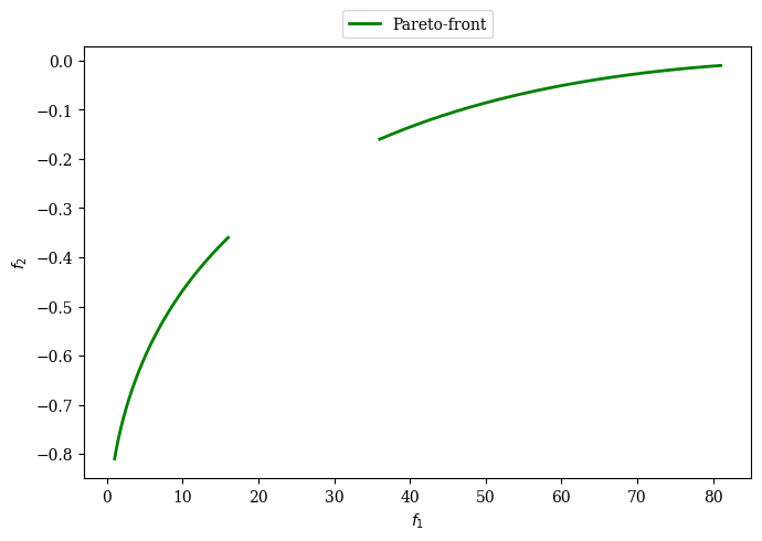
Next, we derive the Pareto-front by mapping the Pareto-set to the objective space. The Pareto-front equation is based on \(f_2\) depending on the variable of \(f_1\). We know that at the optimum \(x_2=0\) which means we can simplify the objective functions to \(f_1(x) = 100 \; x_1^2\) and \(f_2(x) = -(x_1-1)^2\). The first objective \(f_1\) can be reformulated to \(x_1 = \sqrt{\frac{f_1}{100}}\) and then be put into the second objective which results in
The equation defines the shape, however, next all possible values for \(f_1\) need to be defined. As shown before the Pareto-set is defined for \((0.1 \leq x_1 \leq 0.4) \lor (0.6 \leq x_1 \leq 0.9) \, \land \, x_2 = 0\). If we plug in the values for \(x_1\) into \(f_1\) we get the points of interest \([1,16]\) and \([36,81]\). Thus the Pareto-front is given by:
[2]:
import numpy as np
import matplotlib.pyplot as plt

plt.figure(figsize=(7, 5))

f2 = lambda f1: - ((f1/100) ** 0.5 - 1)**2
F1_a, F1_b = np.linspace(1, 16, 300), np.linspace(36, 81, 300)
F2_a, F2_b = f2(F1_a), f2(F1_b)

plt.rc('font', family='serif')
plt.plot(F1_a,F2_a, linewidth=2.0, color="green", label="Pareto-front")
plt.plot(F1_b,F2_b, linewidth=2.0, color="green")

plt.xlabel("$f_1$")
plt.ylabel("$f_2$")

plt.legend(loc='upper center', bbox_to_anchor=(0.5, 1.10),
          ncol=4, fancybox=True, shadow=False)

plt.tight_layout()
plt.show()

As a quick check, we shall verify if this is a non-dominated set. Keeping in mind that the first objective is minimized and the second maximized for this optimization problem, a better solution lies on the top left. This means the derived Pareto-front makes sense.
Hint
Researchers have developed all kinds of test problems and derived their optima from designing and comparing suitable optimization algorithms. However, deriving the Pareto-set and Pareto-front from a mathematical problem formulation can become quite challenging for more complicated problems or not even be possible. Also, not all algorithms can be put into a math equation and might be of a black-box nature. Thus, we use optimization algorithms to find (near-optimal) solutions using well-benchmarked algorithms.