Callback¶

A Callback class can be used to receive a notification of the algorithm object each generation. This can be useful to track metrics, do additional calculations, or even modify the algorithm object during the run. The latter is only recommended for experienced users.

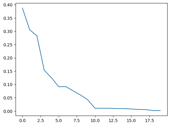
The example below implements a less memory-intense version of keeping track of the convergence. A posteriori analysis can one the one hand, be done by using the save_history=True option. This, however, stores a deep copy of the Algorithm object in each iteration. This might be more information than necessary, and thus, the Callback allows to select only the information necessary to be analyzed when the run has terminated. Another good use case can be to visualize data in each iteration in real-time.

Tip

The callback has full access to the algorithm object and thus can also alter it. However, the callback’s purpose is not to customize an algorithm but to store or process data.

[1]:

import matplotlib.pyplot as plt
import numpy as np

from pymoo.algorithms.soo.nonconvex.ga import GA
from pymoo.problems import get_problem
from pymoo.core.callback import Callback
from pymoo.optimize import minimize


class MyCallback(Callback):

    def __init__(self) -> None:
        super().__init__()
        self.data["best"] = []

    def notify(self, algorithm):
        self.data["best"].append(algorithm.pop.get("F").min())


problem = get_problem("sphere")

algorithm = GA(pop_size=100)

res = minimize(problem,
               algorithm,
               ('n_gen', 20),
               seed=1,
               callback=MyCallback(),
               verbose=True)

val = res.algorithm.callback.data["best"]
plt.plot(np.arange(len(val)), val)
plt.show()

=================================================================
n_gen  |  n_eval  |     f_avg     |     f_min     |     f_gap
=================================================================
     1 |      100 |  0.8314974785 |  0.3870993357 |  0.3870993357
     2 |      200 |  0.5715705191 |  0.3057138275 |  0.3057138275
     3 |      300 |  0.4550327555 |  0.2411375542 |  0.2411375542
     4 |      400 |  0.3660527555 |  0.2155814787 |  0.2155814787
     5 |      500 |  0.2947869167 |  0.1341235205 |  0.1341235205
     6 |      600 |  0.2294618212 |  0.0976818958 |  0.0976818958
     7 |      700 |  0.1695381744 |  0.0427806264 |  0.0427806264
     8 |      800 |  0.1220873448 |  0.0229230788 |  0.0229230788
     9 |      900 |  0.0859605984 |  0.0229230788 |  0.0229230788
    10 |     1000 |  0.0602567663 |  0.0205097034 |  0.0205097034
    11 |     1100 |  0.0438274420 |  0.0101914617 |  0.0101914617
    12 |     1200 |  0.0306870814 |  0.0101914617 |  0.0101914617
    13 |     1300 |  0.0218382714 |  0.0088134417 |  0.0088134417
    14 |     1400 |  0.0155204754 |  0.0064739505 |  0.0064739505
    15 |     1500 |  0.0113980792 |  0.0055368760 |  0.0055368760
    16 |     1600 |  0.0090963003 |  0.0045096334 |  0.0045096334
    17 |     1700 |  0.0074727464 |  0.0043313289 |  0.0043313289
    18 |     1800 |  0.0060336312 |  0.0029932195 |  0.0029932195
    19 |     1900 |  0.0050404559 |  0.0029932195 |  0.0029932195
    20 |     2000 |  0.0043911966 |  0.0026475866 |  0.0026475866

Note that the Callback object from the Result object needs to be accessed res.algorithm.callback because the original object keeps unmodified to ensure reproducibility.

For completeness, the history-based convergence analysis looks as follows:

[2]:

res = minimize(problem,
               algorithm,
               ('n_gen', 20),
               seed=1,
               save_history=True)

val = [e.opt.get("F")[0] for e in res.history]
plt.plot(np.arange(len(val)), val)
plt.show()