ZDT

The ZDT [5] problem suite is based on the construction process

\begin{align} \begin{split} \min && \; f_1(x)\\[2mm] \min && \; f_2(x) = g(x) \, h(f_1(x),g(x)) \end{split} \end{align}

where two objective have to be minimized. The function \(g(x)\) can be considered as the function for convergence and usually \(g(x) = 1\) holds for pareto-optimal solutions (except for ZDT5).

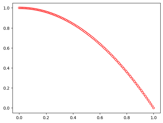
ZDT1

This is a 30-variable problem (\(n=30\)) with a convex Pareto-optimal set:

Definition

\begin{align} \begin{split} f_1(x) &= \, & x_1 \\ g(x) &=& 1 + \frac{9}{n-1} \; \sum_{i=2}^{n} x_i \\ h(f_1,g) &=& 1 - \sqrt{f_1/g} \\ \end{split} \end{align}

\[0 \leq x_i \leq 1 \quad i=1,\ldots,n\]

Optimum

\[0 \leq x_1^* \leq 1 \quad \text{and} \quad x_i^*=0 \; \text{for} \; i=2,\ldots,n\]

Plot

from pymoo.problems import get_problem
from pymoo.visualization.util import plot

problem = get_problem("zdt1")
plot(problem.pareto_front(), no_fill=True)

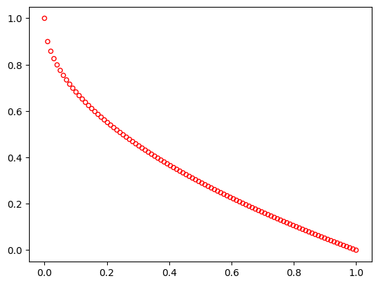
ZDT2

This is also a 30-variable problem (\(n=30\)) with a non-convex Pareto-optimal set:

Definition

\begin{align} \begin{split} f_1(x) &= \, & x_1 \\ g(x) &=& 1 + \frac{9}{n-1} \; \sum_{i=2}^{n} x_i \\ h(f_1,g) &=& 1 - (f_1/g)^2 \\ \end{split} \end{align}

\[0 \leq x_i \leq 1 \quad i=1,\ldots,n\]

Optimum

\[0 \leq x_1^* \leq 1 \quad \text{and} \quad x_i^*=0 \; \text{for} \; i=2,\ldots,n\]

Plot

from pymoo.problems import get_problem
from pymoo.visualization.util import plot

problem = get_problem("zdt2")
plot(problem.pareto_front(), no_fill=True)

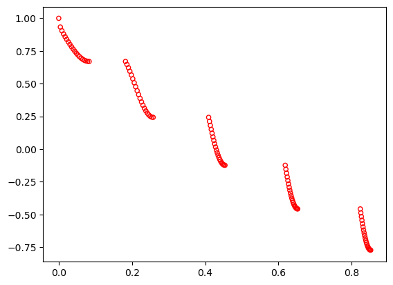
ZDT3

This is also a 30-variable problem (\(n=30\)) with a number of disconnected Pareto-optimal fronts:

Definition

\begin{align} \begin{split} f_1(x) &= \, & x_1 \\ g(x) &=& 1 + \frac{9}{n-1} \; \sum_{i=2}^{n} x_i \\ h(f_1,g) &=& 1 - \sqrt{f_1/g} - (f_1/g) \; \sin(10\pi f_1)\\ \end{split} \end{align}

\[0 \leq x_i \leq 1 \quad i=1,\ldots,n\]

Optimum

\[\begin{split}0 \leq x_1^* \leq 0.0830 \\ 0.1822 \leq x_1^* \leq 0.2577\\ 0.4093 \leq x_1^* \leq 0.4538 \\ 0.6183 \leq x_1^* \leq 0.6525 \\ 0.8233 \leq x_1^* \leq 0.8518 \\ x_i^*=0 \; \text{for} \; i=2,\ldots,n\end{split}\]

Plot

from pymoo.problems import get_problem
from pymoo.visualization.util import plot

problem = get_problem("zdt3")
plot(problem.pareto_front(), no_fill=True)

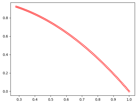
ZDT4

This is a 10-variable (\(n=10\)) problem having a convex Pareto-optimal set. There exist many local Pareto-optimal solutions in this problem. Therefore, algorithms can easily get stuck in a local optimum.

Definition

\begin{align} \begin{split} f_1(x) &= \, & x_1 \\ g(x) &=& 1 + 10(n-1) + \sum_{i=2}^{n} (x_i^2 - 10 \cos(4\pi x_i))\\ h(f_1,g) &=& 1 - \sqrt{f_1/g}\\ \end{split} \end{align}

\[\begin{split}0 \leq x_1 \leq 1 \\ -10 \leq x_i \leq 10 \quad i=2,\ldots,n\end{split}\]

Optimum

\[0 \leq x_1^* \leq 1 \quad \text{and} \quad x_i^*=0 \; \text{for} \; i=2,\ldots,n\]

Plot

from pymoo.problems import get_problem
from pymoo.visualization.util import plot

problem = get_problem("zdt4")
plot(problem.pareto_front(), no_fill=True)

ZDT5

In ZDT5 the variables are decoded by bitstrings. At all 11 discrete variables are used, where \(x_1\) is represented by 30 bits and the rest \(x_2\) to \(x_{11}\) by 5 bits each. The function \(u(x)\) does nothing else than count the number of \(1\) of the corresponding variable. Also, note that the objective function is deceptive, because the values of \(v(u(x_i))\) are decreasing with the number of 1’s, but have their minimum when all variables are indeed 1.

Definition

\begin{align} \begin{split} f_1(x) &= \, & 1+u(x_1)\\ g(x) &=& \sum_{i=2}^{n} v(u(x_i))\\[2mm] v(u(x_i)) &=& \begin{cases} 2 + u(x_i) \quad \text{if} \; u(x_i) < 5\\ 1 \quad \quad \quad \; \; \; \text{if} \; u(x_i) = 5 \end{cases}\\[4mm] h(f_1,g) &=& 1 /f_1(x)\\[2mm] \end{split} \end{align}

Optimum

\[0 \leq u(x_1^*) \leq 30 \quad \text{and} \quad u(x_i^*)=5 \; \text{for} \; i=2,\ldots,n\]

Plot

from pymoo.problems import get_problem
from pymoo.visualization.util import plot

problem = get_problem("zdt5", normalize=False)
plot(problem.pareto_front(), no_fill=True)

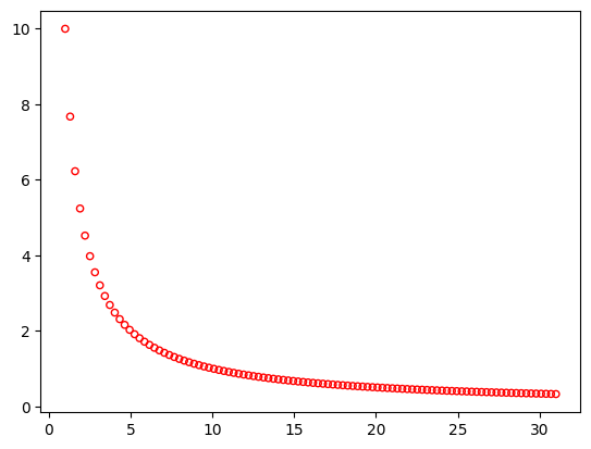
Please note that by default here the Pareto-front is not normalized. However, this can be easily achieved by normalizing \(f_1\) in the range of \((1,31)\) and \(f_2\) in \((10/31, 10)\) which are the known bounds of the Pareto-set. By default the normalized problem is used.

from pymoo.problems import get_problem
from pymoo.visualization.util import plot

problem = get_problem("zdt5", normalize=False)
plot(problem.pareto_front(), no_fill=True)

ZDT6

This is a 10-variable (\(n=10\)) problem having a nonconvex Pareto-optimal set. The density of solutions across the Pareto-optimal region is non-uniform.

Definition

\begin{align} \begin{split} f_1(x) &= \, & 1 - \exp(-4 x_1) \sin^6 (6 \pi x_1) \\[2mm] g(x) &=& 1 + 9 \bigg[\bigg( \sum_{i=2}^{n} x_i \bigg) / 9\bigg]^{0.25}\\[2mm] h(f_1,g) &=& 1 - (f_1/g)^2\\ \end{split} \end{align}

\[0 \leq x_i \leq 1 \quad i=1,\ldots,n\]

Optimum

\[0 \leq x_1^* \leq 1 \quad \text{and} \quad x_i^*=0 \; \text{for} \; i=2,\ldots,n\]

Plot

from pymoo.problems import get_problem
from pymoo.visualization.util import plot

problem = get_problem("zdt6")
plot(problem.pareto_front(), no_fill=True)