GitHub Newsletter Discord

Version: 0.6.1.3

Multi-Criteria Decision Making (MCDM)

The focus of pymoo is on optimization methods itself. However, some basic multi-criteria decision making methods are available:

Compromise Programming

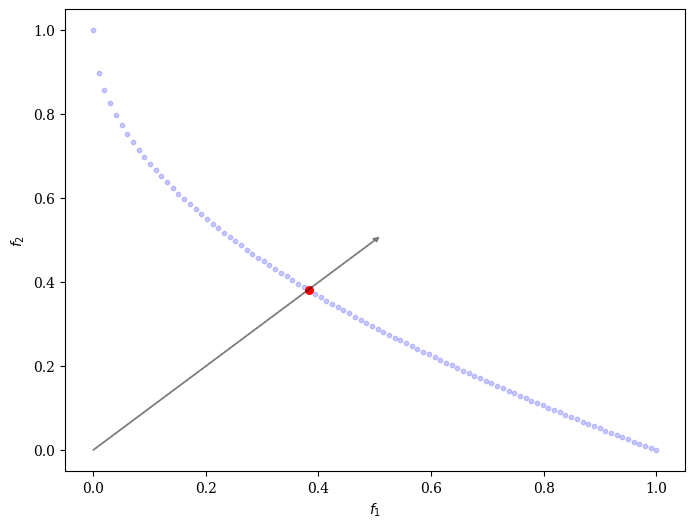
We can use any scalarization method and use it for post-processing. Let us assume our algorithm has converged to the Pareto-front:

from pymoo.problems import get_problem

F = get_problem("zdt1").pareto_front()

Then, we initialize weights and our decomposition function:

import numpy as np

from pymoo.decomposition.asf import ASF

weights = np.array([0.5, 0.5])
decomp = ASF()

We apply the decomposition and retrieve the best value (here minimum):

I = decomp(F, weights).argmin()
print("Best regarding decomposition: Point %s - %s" % (I, F[I]))

Best regarding decomposition: Point 38 - [0.38383838 0.38045308]

Visualize it:

from pymoo.visualization.scatter import Scatter

plot = Scatter()
plot.add(F, color="blue", alpha=0.2, s=10)
plot.add(F[I], color="red", s=30)
plot.do()
plot.apply(lambda ax: ax.arrow(0, 0, 0.5, 0.5, color='black',
                               head_width=0.01, head_length=0.01, alpha=0.4))
plot.show()

<pymoo.visualization.scatter.Scatter at 0x11993ea20>

Pseudo-Weights

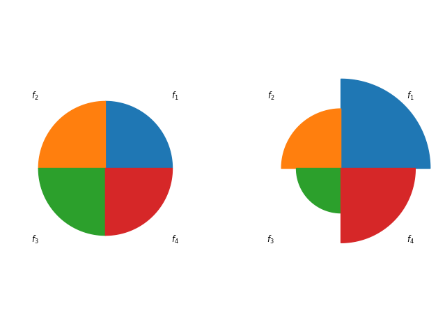
A simple way to chose a solution out of a solution set in the context of multi-objective optimization is the pseudo-weight vector approach proposed in [26]. Respectively, the pseudo weight \(w_i\) for the i-ith objective function can be calculated by:

\begin{equation} w_i = \frac{(f_i^{max} - f_i {(x)}) \, /\, (f_i^{max} - f_i^{min})}{\sum_{m=1}^M (f_m^{max} - f_m (x)) \, /\, (f_m^{max} - f_m^{min})} \end{equation}

This equation calculates the normalized distance to the worst solution regarding each objective \(i\). Please note that for non-convex Pareto fronts the pseudo weight does not correspond to the result of an optimization using the weighted sum. However, for convex Pareto-fronts the pseudo weights are an indicator of the location in the objective space.

from pymoo.mcdm.pseudo_weights import PseudoWeights
from pymoo.util.ref_dirs import get_reference_directions
from pymoo.visualization.petal import Petal

ref_dirs = get_reference_directions("das-dennis", 4, n_partitions=12)
F = get_problem("dtlz1").pareto_front(ref_dirs)

weights = np.array([0.25, 0.25, 0.25, 0.25])
a, pseudo_weights = PseudoWeights(weights).do(F, return_pseudo_weights=True)

weights = np.array([0.4, 0.20, 0.15, 0.25])
b, pseudo_weights = PseudoWeights(weights).do(F, return_pseudo_weights=True)

plot = Petal(bounds=(0, 0.5), reverse=True)
plot.add(F[[a, b]])
plot.show()

<pymoo.visualization.petal.Petal at 0x11b1fbbc0>

High Trade-off Points

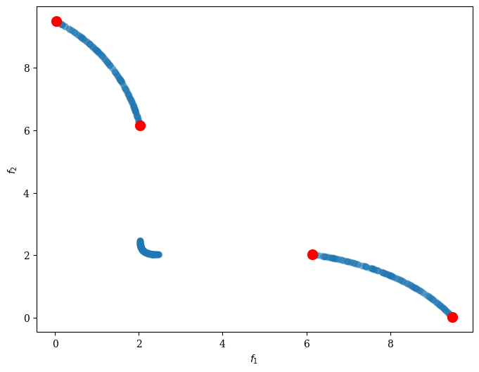
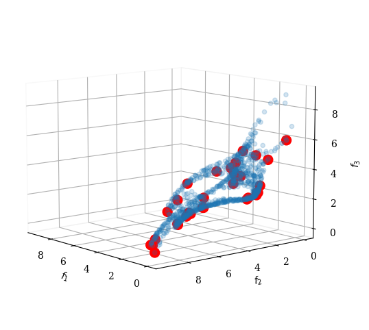
Furthermore, high trade-off points are usually of interest. We have implemented the trade-off metric proposed in [28]. An example for 2 and 3 dimensional solution is given below:

import os

import numpy as np
from pymoo.visualization.scatter import Scatter
from pymoo.mcdm.high_tradeoff import HighTradeoffPoints

pf = np.loadtxt("knee-2d.out")
dm = HighTradeoffPoints()

I = dm(pf)

plot = Scatter()
plot.add(pf, alpha=0.2)
plot.add(pf[I], color="red", s=100)
plot.show()

<pymoo.visualization.scatter.Scatter at 0x11b3a8320>

pf = np.loadtxt("knee-3d.out")

I = dm(pf)

plot = Scatter(angle=(10, 140))
plot.add(pf, alpha=0.2)
plot.add(pf[I], color="red", s=100)
plot.show()

<pymoo.visualization.scatter.Scatter at 0x11b26aa20>

<< Video

Case Studies >>