Karush Kuhn Tucker Proximity Measure (KKTPM)

In 2016, Deb and Abouhawwash proposed Karush Kuhn Tucker Proximity Measure (KKTPM) [57], a metric that can measure how close a point is from being “an optimum”. The smaller the metric, the closer the point. This does not require the Pareto front to be known, but the gradient information needs to be approximated. Their metric applies to both single objective and multi-objective optimization problems.

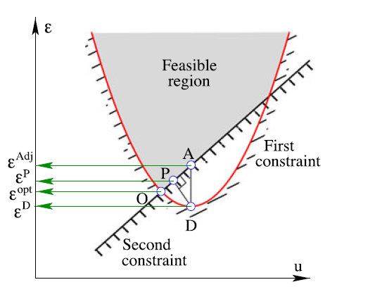
In a single objective problem, the metric shows how close a point is from being a “local optimum”, while in multi-objective problems, the metric shows how close a point is from being a “local Pareto point”. Exact calculations of KKTPM for each point requires solving a whole optimization problem, which is extremely time-consuming. To avoid this problem, the authors of the original work again proposed several approximations to the true KKTPM, namely Direct KKTPM, Projected KKTPM, Adjusted KKTPM, and Approximate KKTPM. Approximate KKTPM is simply the average of the former three and is what we call simply “KKTPM”. Moreover, they were able to show that Approximate KKTPM is reliable and can be used in place of the exact one [58].

Let us now see how to use pymoo to calculate the KKTPM for a point:

from pymoo.constraints.from_bounds import ConstraintsFromBounds
from pymoo.gradient.automatic import AutomaticDifferentiation
from pymoo.problems import get_problem

problem = AutomaticDifferentiation(ConstraintsFromBounds(get_problem("zdt1", n_var=30)))

For instance, the code below calculates the KKTPM metric for randomly sampled points for the given example:

from pymoo.indicators.kktpm import KKTPM
from pymoo.operators.sampling.rnd import FloatRandomSampling

X = FloatRandomSampling().do(problem, 100).get("X")
kktpm = KKTPM().calc(X, problem)

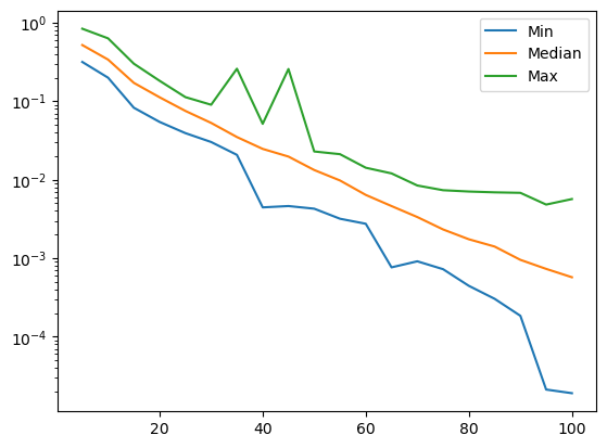
Moreover, a whole run of a genetic algorithm can be analyzed by storing each generation’s history and then calculating the KKTPM metric for each of the points:

from pymoo.algorithms.moo.nsga2 import NSGA2
from pymoo.problems import get_problem
from pymoo.optimize import minimize
from pymoo.visualization.scatter import Scatter
from pymoo.core.evaluator import Evaluator


algorithm = NSGA2(pop_size=100, eliminate_duplicates=True)

# make sure each evaluation also has the derivatives - necessary for KKTPM
evaluator = Evaluator(evaluate_values_of=["F", "G", "dF", "dG"])

res = minimize(problem,
               algorithm,
               ('n_gen', 100),
               evaluator=evaluator,
               seed=1,
               save_history=True,
               verbose=False)

import pandas as pd
import numpy as np

# Collect KKTPM data for each generation
data = []
for algorithm in res.history:
    if algorithm.n_gen % 5 == 0:
        X = algorithm.pop.get("X")
        kktpm = KKTPM().calc(X, problem)

        # Add each individual's KKTPM value with generation info
        for i, value in enumerate(kktpm):
            data.append({
                'generation': algorithm.n_gen,
                'individual': i,
                'kktpm': value
            })

# Create DataFrame
df = pd.DataFrame(data)
df

	generation	individual	kktpm
0	5	0	0.578128
1	5	1	0.556041
2	5	2	0.481507
3	5	3	0.638571
4	5	4	0.552443
...	...	...	...
1995	100	95	0.006646
1996	100	96	0.007908
1997	100	97	0.011097
1998	100	98	0.007232
1999	100	99	0.009157

2000 rows × 3 columns

# Get summary statistics for each generation
stats_by_gen = df.groupby('generation')['kktpm'].describe()
stats_by_gen

	count	mean	std	min	25%	50%	75%	max
generation
5	100.0	0.606367	0.102607	0.413505	0.531672	0.601515	0.691302	0.823210
10	100.0	0.437565	0.100178	0.256413	0.352657	0.426188	0.525569	0.625640
15	100.0	0.327390	0.084982	0.199976	0.256976	0.313050	0.392336	0.495058
20	100.0	0.234454	0.073420	0.109959	0.181489	0.200261	0.294889	0.402596
25	100.0	0.184949	0.048054	0.077966	0.152082	0.166390	0.227511	0.295211
30	100.0	0.157165	0.041126	0.063416	0.128238	0.143977	0.190136	0.279304
35	100.0	0.122228	0.033381	0.028348	0.103134	0.112931	0.141745	0.190694
40	100.0	0.100814	0.026641	0.020273	0.083457	0.095660	0.112486	0.166559
45	100.0	0.078313	0.020058	0.019823	0.068038	0.074447	0.086282	0.134496
50	100.0	0.062054	0.013506	0.015916	0.055734	0.059743	0.068355	0.113593
55	100.0	0.047471	0.010750	0.016135	0.039670	0.047031	0.054423	0.071587
60	100.0	0.034896	0.007247	0.012692	0.030444	0.033539	0.038914	0.057769
65	100.0	0.035714	0.039961	0.013633	0.023666	0.029073	0.034778	0.258761
70	100.0	0.022869	0.005775	0.011882	0.018193	0.022407	0.025962	0.039261
75	100.0	0.017109	0.003856	0.009919	0.014264	0.016124	0.019667	0.031376
80	100.0	0.016684	0.024352	0.008281	0.012165	0.013918	0.016429	0.256016
85	100.0	0.012111	0.002707	0.007561	0.010196	0.011751	0.013273	0.021814
90	100.0	0.010202	0.002392	0.005750	0.008470	0.009991	0.011494	0.018209
95	100.0	0.009075	0.002409	0.005070	0.007201	0.008927	0.010152	0.019328
100	100.0	0.007976	0.001966	0.004577	0.006687	0.007807	0.008869	0.014139

import matplotlib.pyplot as plt

# Plot the quartiles and median over generations
generations = stats_by_gen.index
plt.plot(generations, stats_by_gen['25%'], label="Q1 (25th percentile)")
plt.plot(generations, stats_by_gen['50%'], label="Median")
plt.plot(generations, stats_by_gen['75%'], label="Q3 (75th percentile)")
plt.yscale("log")
plt.xlabel("Generation")
plt.ylabel("KKTPM")
plt.title("KKTPM Statistics Over Generations")
plt.legend()
plt.grid(True, alpha=0.3)
plt.show()